Why Carbon Maps Disagree – and How to Choose the Right One

Carbon maps don’t agree. Two products covering the same forest, at the same time, can differ by 100% or more on estimated biomass. That’s the predictable result of different modelling approaches, calibration strategies, and underlying assumptions.

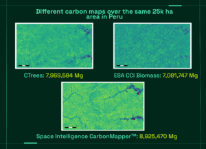
In the example above, the carbon values differ by as much as 26%, with the Space Intelligence’s CarbonMapper detecting higher biomass overall. That is because this map also features more detail and more variation, and lower biomass forest and cleared areas near rivers are more obvious.

If you’re evaluating a project portfolio for credibility, even a 26% over- or under-estimate in baseline carbon stocks means either leaving credits on the table, or inflating credit projections and subsequent reputational exposure.

So what contributes to this difference and how do you minimise risk when choosing a data provider for your project? Not all maps are built for the job they’re being asked to do. The market offers 4 fundamentally different approaches to carbon mapping, each with different strengths, limitations, and appropriate use cases. Understanding what separates them is the first step to making a defensible choice.

Why do carbon maps disagree?

A carbon map estimates the mass of carbon stored in forest biomass – typically expressed as aboveground biomass (AGB) in tonnes per hectare. What separates products isn’t the raw satellite data, which is largely the same across providers. It’s what they do with it.

Two key choices drive most of the disagreement:

• Calibration. A model trained on global data produces global predictions. A model calibrated to local field plots, allometric equations, and biome-specific conditions produces local predictions. Global models can under- or over-estimate biomass in some forest types by 100% or more – not because they’re poorly built, but because they weren’t built for that specific forest.
• Uncertainty. Most products report how accurate their map is at a single point in time. Very few report the uncertainty on change over time – which is the only number that matters for credit issuance. 

The four approaches

Understanding the disagreement starts with understanding that there are four distinct approaches to carbon mapping – and each one is suited to a different stage of the carbon project lifecycle.

Approach 1: Field plots + land cover stratification

The original method. Ground-based forest inventory plots measure biomass directly, and a land cover map extrapolates those values across the wider landscape. This approach underpins national inventories and many REDD+ carbon calculations (VM0007, VM0010, VM0048). It’s reliable and well-understood – but it cannot detect within-class variation. A stratum labelled “dense forest” gets one average value, whether individual areas contain 80 or 280 Mg AGB/ha.

Best for: national inventories, VM0007/VM0010/VM0048 carbon impact calculations, low-budget pre-feasibility. 

Not for: spatially explicit AGB, degradation monitoring, or contexts requiring uncertainty of change within-strata.

 

Approach 2: Global LiDAR-trained models

NASA’s GEDI and ICESat-2 satellites provide canopy height measurements globally. These train machine learning models against wall-to-wall satellite imagery, producing AGB estimates at every pixel – globally, at 10-30m resolution. The result is the most accessible and widely used category of carbon maps on the market today.

Their strength is coverage and cost. Their limitation is the same as any global model: they weren’t calibrated to your specific forest. They’re built for screening, not for credit issuance.

Used for: portfolio screening, pre-feasibility, non-VCM reporting (TNFD, Scope 3 FLAG), baselines under Equitable Earth’s REDD+ standard M002, feasibility studies under Isometric. 

Not for: baselines under VM0047, VM0048, Isometric, or EE M001 – most current methodologies require locally calibrated AGB.

Providers in this category include: Planet Forest Carbon Diligence, Chloris, Sylvera Biomass Atlas, CTrees, Kanop, Space Intelligence GHL.

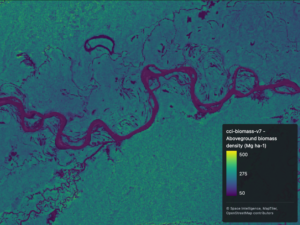
Approach 3: Project-level calibrated models

Same inputs as Approach 2 – LiDAR-derived canopy height plus optical and radar imagery – but the model is trained and calibrated specifically to the project region, using local field data and allometric equations. The difference in output quality is significant: local calibration reduces systematic bias, enables degradation detection within forest classes, and makes uncertainty of change quantifiable.

This is the approach that qualifies as audit-grade – meaning it meets the requirements of the highest integrity new generation carbon standards like Isometric and Equitable Earth M001, and Verra’s VM0045. It costs more and takes longer than a global product. It is not overkill if you need to enable high quality credit issuance.

Best for: credit issuance baselines, investment-grade due diligence, annual MRV.

Limitations: higher cost and lead time; field data required (not necessarily from project site; from the surrounding region is sufficient).

Space Intelligence’s CarbonMapper sits in this category.

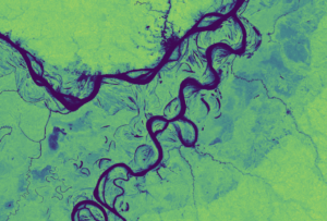
Approach 4: Radar / optical proxy models

Radar backscatter (SAR) or optical vegetation indices serve as proxies for forest structure and biomass. They can be locally calibrated to perform very well at estimating the carbon stored in growing trees. The SAR  approaches are particularly suited to cloud-prone environments, and in general have more consistency than optical datasets between seasons and years. Different SAR wavelengths are available, with Sentinel-1 at C-band (~6 cm) and JAXA’s ALOS-2 PALSAR-2 and NASA/ISRO’s NISAR at L-band (~20cm) best for lower and mid-biomass systems, and ESA’s BIOMASS satellite – launched in 2025 – using P-band SAR (60cm), ideal for high biomass tropical forests. 

Best for:  stocking index-based reforestation methodologies (VM0047), short vegetation and agroforestry. 

Not for: dense forest above ~150 Mg/ha (radar saturates), or AGB-explicit methodology baselines.

So, which one should you use?

Ultimately, it comes down to two factors: your project’s current stage and your chosen methodology. While a global LiDAR-trained product is an excellent tool for rapidly screening a pipeline of 50 potential sites, it falls short when you need to establish a precise baseline for a single project.

If you need high-quality, rigorously accurate carbon mapping for your project site, contact our team today.